Jupyter (IPython) notebooks features
Jupyter (IPython) notebooks features
It is very flexible tool to create readable analyses, because one can keep code, images, comments, formula and plots together:
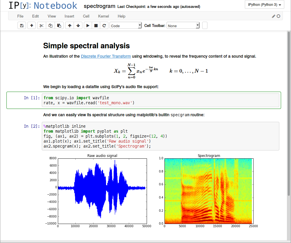
Jupyter is quite extensible, supports many programming languages, easily hosted on almost any server — you only need to have ssh or http access to a server. And it is completely free.
Basics
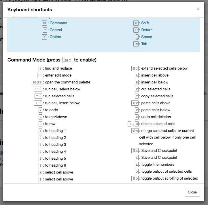
List of hotkeys is shown in Help > Keyboard Shortcuts (list is extended from time to time, so don't hesitate to look at it again).
This gives an idea of how you're expected to interact with notebook. If you're using notebook constantly, you'll of course learn most of the list. In particular:
Esc + FFind and replace to search only over the code, not outputsEsc + OToggle cell output- You can select several cells in a row and delete / copy / cut / paste them. This is helpful when you need to move parts of a notebook
Sharing notebooks
Simplest way is to share notebook file (.ipynb), but not everyone is using notebooks, so the options are
- convert notebooks to html file
- share it with gists, which are rendering the notebooks. See this example
- store your notebook e.g. in dropbox and put the link to nbviewer. nbviewer will render the notebook
- github renders notebooks (with some limitations, but in most cases it is ok), which makes it very useful to keep history of your research (if research is public)
Plotting in notebooks
There are many plotting options:
- matplotlib (de-facto standard), activated with
%matplotlib inline %matplotlib notebookis interactive regime, but very slow, since rendering is done on server-side.- mpld3 provides alternative renderer (using d3) for matplotlib code. Quite nice, though incomplete
- bokeh is a better option for building interactive plots
- plot.ly can generate nice plots, but those will cost you money

Magics
Magics are turning simple python into magical python. Magics are the key to power of ipython.
# list available python magics
%lsmagic
%env
You can manage environment variables of your notebook without restarting the jupyter server process. Some libraries (like theano) use environment variables to control behavior, %env is the most convenient way.
# %env - without arguments lists environmental variables
%env OMP_NUM_THREADS=4
Executing shell commands
You can call any shell command. This in particular useful to manage your virtual environment.
!pip install numpy
!pip list | grep Theano
Suppress output of last line
sometimes output isn't needed, so we can either use pass instruction on new line or semicolon at the end
%matplotlib inline
from matplotlib import pyplot as plt
import numpy
# if you don't put semicolon at the end, you'll have output of function printed
plt.hist(numpy.linspace(0, 1, 1000)**1.5);

See the source of python functions / classes / whatever with question mark (?, ??)
from sklearn.cross_validation import train_test_split
# show the sources of train_test_split function in the pop-up window
train_test_split??
# you can use ? to get details about magics, for instance:
%pycat?
will output in the pop-up window:
Show a syntax-highlighted file through a pager.

This magic is similar to the cat utility, but it will assume the file
to be Python source and will show it with syntax highlighting.

This magic command can either take a local filename, an url,
an history range (see %history) or a macro as argument ::

%pycat myscript.py
%pycat 7-27
%pycat myMacro
%pycat http://www.example.com/myscript.py
%run to execute python code
%run can execute python code from .py files — this is a well-documented behavior.
But it also can execute other jupyter notebooks! Sometimes it is quite useful.
NB. %run is not the same as importing python module.
# this will execute all the code cells from different notebooks
%run ./2015-09-29-NumpyTipsAndTricks1.ipynb


%load
loading code directly into cell. You can pick local file or file on the web.
After uncommenting the code below and executing, it will replace the content of cell with contents of file.
# %load http://matplotlib.org/mpl_examples/pylab_examples/contour_demo.py
%store: lazy passing data between notebooks
data = 'this is the string I want to pass to different notebook'
%store data
del data # deleted variable
# in second notebook I will use:
%store -r data
print data
%who: analyze variables of global scope
# pring names of string variables
%who str
Timing
When you need to measure time spent or find the bottleneck in the code, ipython comes to the rescue.
%%time
import time
time.sleep(2) # sleep for two seconds
# measure small code snippets with timeit !
import numpy
%timeit numpy.random.normal(size=100)
%%writefile pythoncode.py

import numpy
def append_if_not_exists(arr, x):
    if x not in arr:
        arr.append(x)

def some_useless_slow_function():
    arr = list()
    for i in range(10000):
        x = numpy.random.randint(0, 10000)
        append_if_not_exists(arr, x)
# shows highlighted source of the newly-created file
%pycat pythoncode.py
from pythoncode import some_useless_slow_function, append_if_not_exists
Profiling: %prun, %lprun, %mprun
# shows how much time program spent in each function
%prun some_useless_slow_function()
Example of output:
26338 function calls in 0.713 seconds

   Ordered by: internal time

   ncalls  tottime  percall  cumtime  percall filename:lineno(function)
    10000    0.684    0.000    0.685    0.000 pythoncode.py:3(append_if_not_exists)
    10000    0.014    0.000    0.014    0.000 {method 'randint' of 'mtrand.RandomState' objects}
        1    0.011    0.011    0.713    0.713 pythoncode.py:7(some_useless_slow_function)
        1    0.003    0.003    0.003    0.003 {range}
     6334    0.001    0.000    0.001    0.000 {method 'append' of 'list' objects}
        1    0.000    0.000    0.713    0.713 <string>:1(<module>)
1 0.000 0.000 0.000 0.000 {method 'disable' of '_lsprof.Profiler' objects}%load_ext memory_profiler
# tracking memory consumption (show in the pop-up)
%mprun -f append_if_not_exists some_useless_slow_function()
Example of output:
Line #    Mem usage    Increment   Line Contents
================================================
     3     20.6 MiB      0.0 MiB   def append_if_not_exists(arr, x):
     4     20.6 MiB      0.0 MiB       if x not in arr:
     5     20.6 MiB      0.0 MiB           arr.append(x)
%lprun is line profiling, but it seems to be broken for latest IPython release, so we'll manage without magic this time:
import line_profiler
lp = line_profiler.LineProfiler()
lp.add_function(some_useless_slow_function)
lp.runctx('some_useless_slow_function()', locals=locals(), globals=globals())
lp.print_stats()
#%%debug filename:line_number_for_breakpoint
# Here some code that fails. This will activate interactive context for debugging
A bit easier option is %pdb, which activates debugger when exception is raised:
# %pdb

# def pick_and_take():
#     picked = numpy.random.randint(0, 1000)
#     raise NotImplementedError()

# pick_and_take()
Writing formulae in latex
markdown cells render latex using MathJax.
$$ P(A \mid B) = \frac{P(B \mid A) \, P(A)}{P(B)} $$Markdown is an important part of notebooks, so don't forget to use its expressiveness!
Using different languages inside single notebook
If you're missing those much, using other computational kernels:
- %%python2
- %%python3
- %%ruby
- %%perl
- %%bash
- %%R
is possible, but obviously you'll need to setup the corresponding kernel first.
%%ruby
puts 'Hi, this is ruby.'
%%bash
echo 'Hi, this is bash.'
Big data analysis
A number of solutions are available for querying/processing large data samples:
- ipyparallel (formerly ipython cluster) is a good option for simple map-reduce operations in python. We use it in rep to train many machine learning models in parallel
- pyspark
- spark-sql magic %%sql
Let others to play with your code without installing anything
Services like mybinder give an access to machine with jupyter notebook with all the libraries installed, so user can play for half an hour with your code having only browser.
You can setup your own system with jupyterhub, this is very handy when you organize mini-course or workshop and don't have time to care about students machines.
Writing functions in other languages
Sometimes the speed of numpy is not enough and I need to write some fast code. In principle, you can compile function in the dynamic library and write python wrappers...
But it is much better when this boring part is done for you, right?
You can write functions in cython or fortran and use those directly from python code.
First you'll need to install:
!pip install cython fortran-magic%load_ext Cython
%%cython
def myltiply_by_2(float x):
    return 2.0 * x
myltiply_by_2(23.)
Personally I prefer to use fortran, which I found very convenient for writing number-crunching functions. More details of usage can be found here.
%load_ext fortranmagic
%%fortran
subroutine compute_fortran(x, y, z)
    real, intent(in) :: x(:), y(:)
    real, intent(out) :: z(size(x, 1))

    z = sin(x + y)

end subroutine compute_fortran
compute_fortran([1, 2, 3], [4, 5, 6])
I also should mention that there are different jitter systems which can speed up your python code. More examples in my notebook.
Multiple cursors
Since recently jupyter supports multiple cursors (in a single cell), just like sublime ot intelliJ!
Gif taken from http://swanintelligence.com/multi-cursor-in-jupyter.html
Jupyter-contrib extensions
are installed with
!pip install https://github.com/ipython-contrib/jupyter_contrib_nbextensions/tarball/master
!pip install jupyter_nbextensions_configurator
!jupyter contrib nbextension install --user
!jupyter nbextensions_configurator enable --user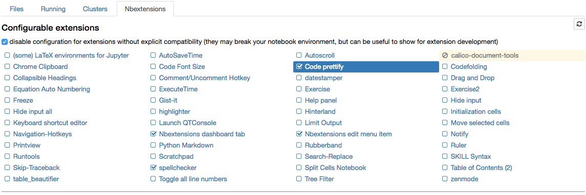
this is a family of different extensions, including e.g. jupyter spell-checker and code-formatter, that are missing in jupyter by default.
RISE: presentations with notebook
Extension by Damian Avila makes it possible to show notebooks as demonstrations. Example of such presentation: http://bollwyvl.github.io/live_reveal/#/7
It is very useful when you teach others e.g. to use some library.
Jupyter output system
Notebooks are displayed as HTML and the cell output can be HTML, so you can return virtually anything: video/audio/images.
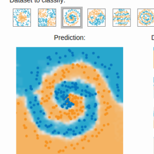
In this example I scan the folder with images in my repository and show first five of them:
import os
from IPython.display import display, Image
names = [f for f in os.listdir('../images/ml_demonstrations/') if f.endswith('.png')]
for name in names[:5]:
    display(Image('../images/ml_demonstrations/' + name, width=300))


I could take the same list with a bash command
because magics and bash calls return python variables:
names = !ls ../images/ml_demonstrations/*.png
names[:5]
Reconnect to kernel
Long before, when you started some long-taking process and at some point your connection to ipython server dropped, you completely lost the ability to track the computations process (unless you wrote this information to file). So either you interrupt the kernel and potentially lose some progress, or you wait till it completes without any idea of what is happening.
Reconnect to kernel option now makes it possible to connect again to running kernel without interrupting computations and get the newcoming output shown (but some part of output is already lost).
Write your posts in notebooks
Like this one. Use nbconvert to export them to html.
Useful links
- IPython built-in magics
- Nice interactive presentation about jupyter by Ben Zaitlen
- Advanced notebooks part 1: magics and part 2: widgets
- Profiling in python with jupyter
- 4 ways to extend notebooks
- IPython notebook tricks
- Jupyter vs Zeppelin for big data
This post was written in IPython. You can download the notebook from repository.
 Gradient boosting
 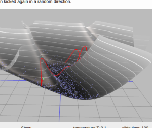 Hamiltonian MC
 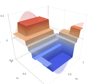 Gradient boosting
  Reconstructing pictures
 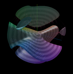 Neural Networks