Reconstructing pictures with machine learning [demonstration]
Reconstructing pictures with machine learning [demonstration]
In this post I demonstrate how different techniques of machine learning are working.
The idea is very simple:
- each black & white image can be treated as a function of 2 variables - x1 and x2, position of a pixel
- intensity of a pixel is output
- this 2-dimentional function is very complex
- we can leave only a small fraction of pixels, treating others as 'lost'
- by looking how different regression algorithms reconstruct the picture, we can get some understanding of how these algorithms are operating
Don't treat this demonstration as some 'comparison of approaches', because this problem (reconstructing a picture) is very specific and has very few in common with typical ML datasets and problems. And of course, this approach is not to be used in practice to reconstruct pictures :)
I am using scikit-learn and making use of its API, enabling user to construct new models via meta-ensembling and pipelines.
First, we import lots of things
# !pip install image
from PIL import Image
%pylab inline
import numpy
from sklearn.pipeline import make_pipeline
from sklearn.ensemble import RandomForestRegressor, BaggingRegressor, GradientBoostingRegressor, AdaBoostRegressor
from sklearn.cross_validation import train_test_split
from sklearn.random_projection import GaussianRandomProjection
from sklearn.tree import DecisionTreeRegressor
from sklearn.linear_model import LinearRegression
from sklearn.kernel_approximation import RBFSampler
from sklearn.preprocessing import StandardScaler
from sklearn.svm import SVR
from sklearn.neighbors import KNeighborsRegressor
from rep.metaml import FoldingRegressor
from rep.estimators import XGBoostRegressor, TheanetsRegressor
Download the picture
I took quite complex picture with many little details
!wget http://static.boredpanda.com/blog/wp-content/uploads/2014/08/cat-looking-at-you-black-and-white-photography-1.jpg -O image.jpg
# !wget http://orig05.deviantart.net/1d93/f/2009/084/5/2/new_york_black_and_white_by_morgadu.jpg -O image.jpg
image = numpy.asarray(Image.open('./image.jpg')).mean(axis=2)
plt.figure(figsize=[20, 10])
plt.imshow(image, cmap='gray')

Define a function to train regressor
train_size is how many pixels shall be used in reconstructing the picture. By default, the algorithm will use only 2% of pixels
def train_display(regressor, image, train_size=0.02):
height, width = image.shape
flat_image = image.reshape(-1)
xs = numpy.arange(len(flat_image)) % width
ys = numpy.arange(len(flat_image)) // width
data = numpy.array([xs, ys]).T
target = flat_image
trainX, testX, trainY, testY = train_test_split(data, target, train_size=train_size, random_state=42)
mean = trainY.mean()
regressor.fit(trainX, trainY - mean)
new_flat_picture = regressor.predict(data) + mean
plt.figure(figsize=[20, 10])
plt.subplot(121)
plt.imshow(image, cmap='gray')
plt.subplot(122)
plt.imshow(new_flat_picture.reshape(height, width), cmap='gray')
Linear regression
not very surprising result
train_display(LinearRegression(), image)

Decision tree limited by depth
train_display(DecisionTreeRegressor(max_depth=10), image)

train_display(DecisionTreeRegressor(max_depth=20), image)

Decision tree limited by minimal number of samples in a leaf
train_display(DecisionTreeRegressor(min_samples_leaf=40), image)

train_display(DecisionTreeRegressor(min_samples_leaf=5), image)

RandomForest
train_display(RandomForestRegressor(n_estimators=100), image)

K Nearest Neighbours
train_display(KNeighborsRegressor(n_neighbors=2), image)

more neighbours + weighting according to distance
to make predictions smoother
train_display(KNeighborsRegressor(n_neighbors=5, weights='distance'), image)

train_display(KNeighborsRegressor(n_neighbors=25, weights='distance'), image)

KNN with canberra metric
train_display(KNeighborsRegressor(n_neighbors=2, metric='canberra'), image)

Gradient Boosting
train_display(XGBoostRegressor(max_depth=5, n_estimators=100, subsample=0.5, nthreads=4), image)

Gradient Boosting with deep trees
train_display(XGBoostRegressor(max_depth=12, n_estimators=100, subsample=0.5, nthreads=4, eta=0.1), image)

Neural networks
neural networks provide smooth predictions and are not able to deal with tiny sharp details of pictures.
train_display(TheanetsRegressor(layers=[20, 20], hidden_activation='tanh',
trainers=[{'algo': 'adadelta', 'learning_rate': 0.01}]), image)

train_display(TheanetsRegressor(layers=[40, 40, 40, 40], hidden_activation='tanh',
trainers=[{'algo': 'adadelta', 'learning_rate': 0.01}]), image)

AdaBoost over Decision Trees using random projections
base = make_pipeline(GaussianRandomProjection(n_components=10),
DecisionTreeRegressor(max_depth=10, max_features=5))
train_display(AdaBoostRegressor(base, n_estimators=50, learning_rate=0.05), image)

Bagging over decision trees using random projections
This is sometimes referred as Random Forest too (since this idea was proposed by Leo Breiman in the same paper).
base = make_pipeline(GaussianRandomProjection(n_components=15),
DecisionTreeRegressor(max_depth=12, max_features=5))
train_display(BaggingRegressor(base, n_estimators=100), image)

See also:
- Drawing an image with deep neural network Andrej Karpathy
- Artificial artist by Tim Head
- Painting photo in different artistic styles. Note that the study in this paper is quite different from things demonstrated in the post.
Feel free to download the notebook from repository and play with other images / parameters.
This post was written in IPython. You can download the notebook from repository.
 Gradient boosting
  Hamiltonian MC
  Gradient boosting
 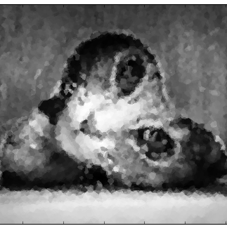 Reconstructing pictures
  Neural Networks