Clustering applied to showers in the OPERA
Abstract: in this post I discuss clustering: techniques that form this method and some peculiarities of using clustering in practice. This post continues previous one about the OPERA.
Update: now you can play with a 3-dimensional visualization of clustering.
What is clustering and when it is needed?
Clustering is a typical problem of unsupervised machine learning. Given a set of objects (also called observations), split them into groups (called clusters) so that objects in each group are more similar to each other than to observations from other groups.
Clustering may become the right tool to identify structure of the data. For instance, cluster analysis helped in 1998 to identify that gamma ray bursts are falling quite nicely in three groups (clusters), not two as was thought before. So we got a hint that there are three types of processes in far galaxies which result in energetic explosions. Now properties of each group can be analyzed individually and we can try to guess processes behind each type of bursts.
Finding groups of users / customers / orders with clustering may turn out to be a good idea (and it may not, there are many factors).
Let me first remind a bit about frequently used clustering methods.
K-means clustering
K-means clustering (wiki) is probably the simplest approach to clustering data. The number of clusters $k$ is predefined, and each cluster is described by its center (mean). Algorithm starts from randomly defined positions of cluster centers, and iteratively refine their positions by repeating the following two steps
- Assignment: each observation is assigned to the cluster with the nearest center
- Update: center of each cluster is updated to the mean of observations in the cluster
You can track the described training process in the following animation:
Limitations of k-means clustering
However this simple algorithm in many cases fails to provide good clustering:
There is a fundamental limitation which prevents k-means from properly clustering above example: k-means clusters are convex polytopes (you can notice this from both demonstrations, but it can be proven quite easily). Moreover, k-means clustering partitions the space into so-called Voronoi diagram.
Another demerit frequently mentioned is that k-means creates clusters of comparable spatial extent and also isn't capable of creating clusters with covariance matrix very different from identity.
DBSCAN
There are more sophisticated approaches to clustering which overcome these limitations of k-means to some extend. One of such methods is DBSCAN (Density-based spatial clustering of applications with noise), which is also quite popular.
The following animation gives some vague understanding about procedure behind DBSCAN clustering:
DBSCAN starts from core points, that is points with several quite close neighbours and creates the cluster by adding closest points. If one of added nearest points is also a core points (has sufficient number of close neighbours), all of its neighbours are also added (and this repeats recursively).
This way DBSCAN is capable of finding complex clusters, quite different in shapes and sizes, but the clusters don't have any parametric description as in other methods (for instance, in k-means cluster is modeled by its center position).
DBSCAN also handles outliers, i.e. observations that do not seem to belong to any clusters. In the clustering of OPERA basetracks that I discuss below it is quite important, as many noise tracks present in the data.
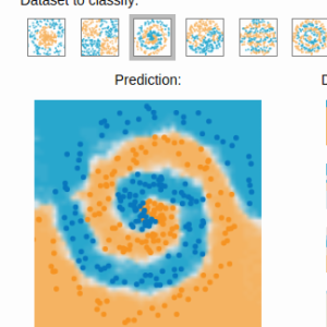
Visual comparison of algorithms in scikit-learn
Scikit-learn package documentation (most popular machine learning package for python) has a very concise and informative visual comparison of different clustering methods:
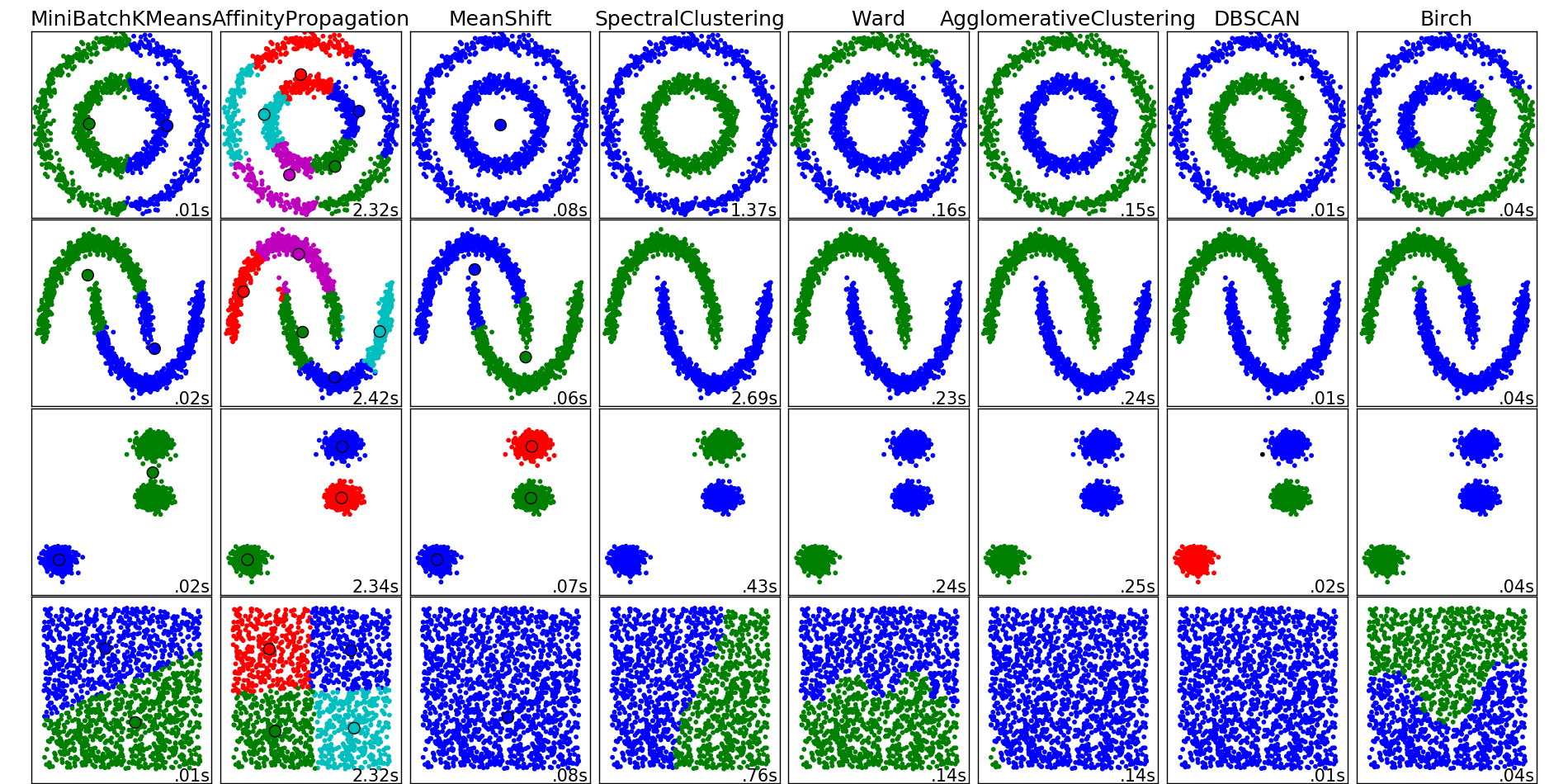
Please refer to that documentation page when in trouble and need to choose the right clustering method for a particular problem.
Back to the OPERA example
Let's now get back to the problem at hand. In the previous post we started from the situation when a brick from the OPERA experiment is developed and scanned. Scanning procedure outputs millions of basetrack, most of which are instrumental background and should be removed.
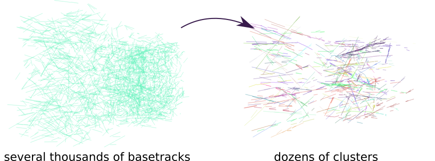
As it was discussed in the previous post, we can clear background and leave only several thousands of tracks thanks to classification techniques and proper feature engineering.
Now we have several thousands tracks and the goal is to find patterns in this data.
Importance of distance choice in applications
Important detail that I want to dwell upon in this post is how do we measure distance between tracks (also called metric function or simply metric). Clustering techniques are unsupervised, and it sounds like they get useful information out of nowhere. Unfortunately, there are no miracles: information is obtained from the structure and provided metric function, which makes it possible to find similarity between items or observations.
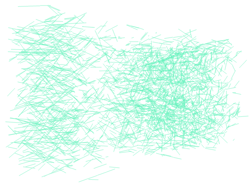
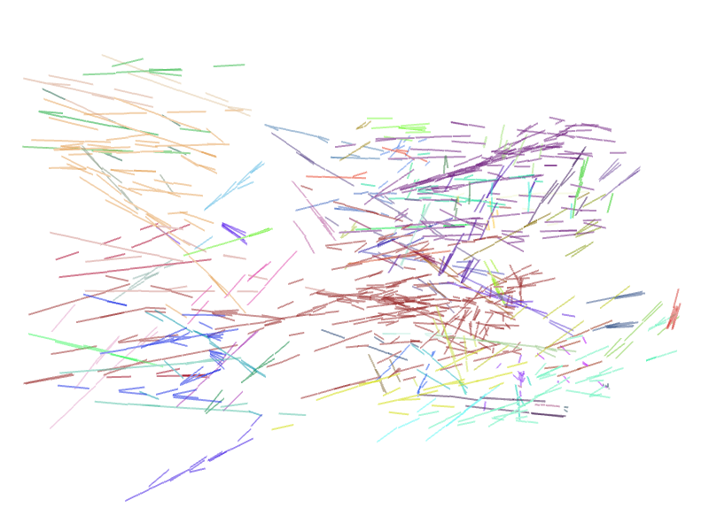
Let's see this in example: what if we simply take euclidean distance and apply DBSCAN clustering? (in this approach we treat each track as a point in 3-dimensional space defined by its position)
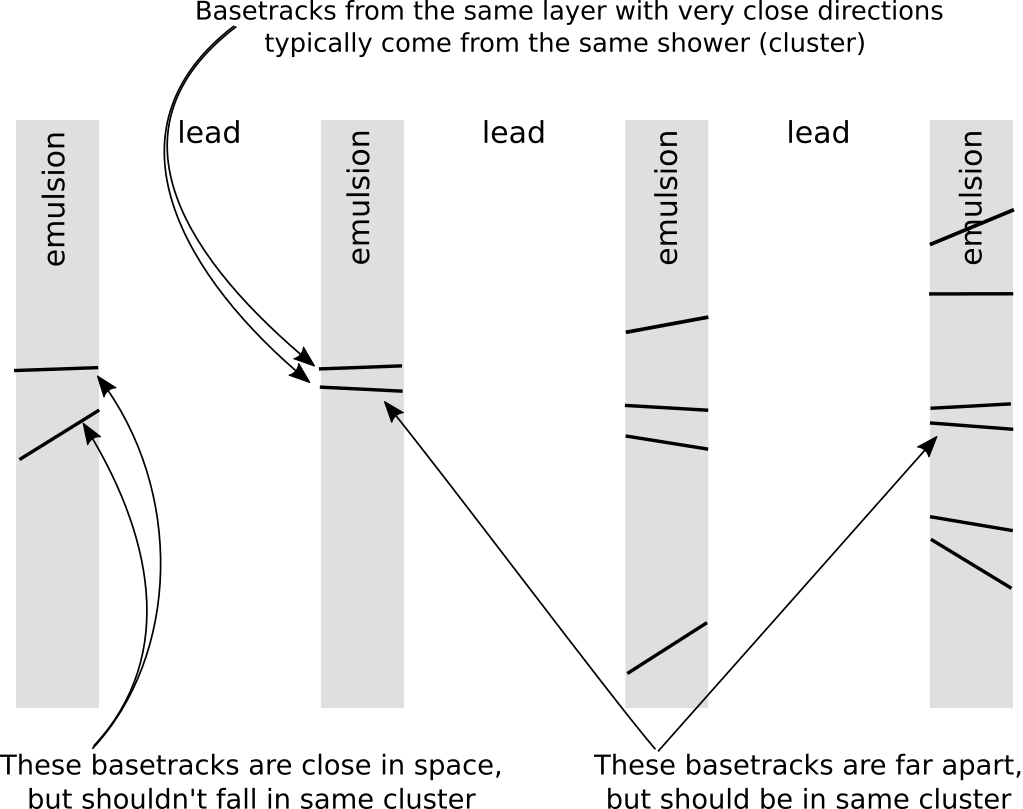
The result is disappointing: found clusters do not correspond to any tracks, those are just groups of tracks placed nearby. An algorithm had no chance to reveal anything useful given the way we defined similarity between tracks. You can see from the scheme below that closest basetracks in euclidean distance rarely belong to the same pattern, while basetracks left by same particle can be quite far from each other:
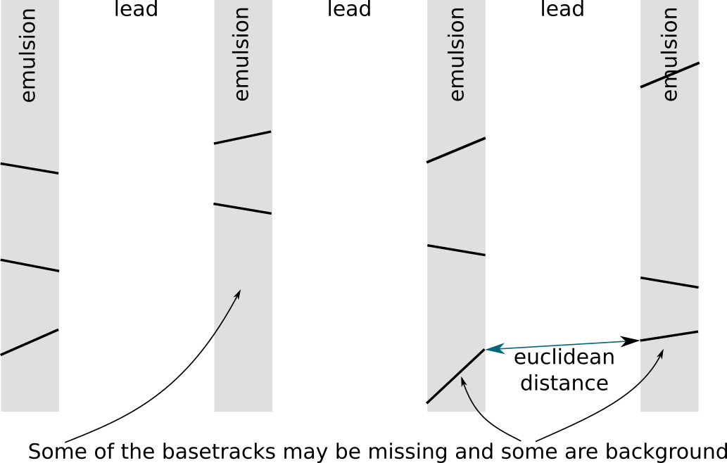
Our clustering should be stable to appearance of noise in the data, in particular noise basetracks that were left in the data should not be attributed to any cluster and marked by algorithm as outliers (DBSCAN handles this situation as was shown in animation).
Another problem in the data is missing links (as shown in the scheme above), when one of the basetracks is missing and algorithm should still consider two parts to the right and to the left as a single pattern. It is problematic, because parts are spaced apart.
Accounting for directions of basetracks
Euclidean distance that we used in previous example can be written as: $$ \rho(\text{track}_1, \text{track}_2)^2 = (x_1 - x_2)^2 + (y_1 - y_2)^2 + (z_1 - z_2)^2, $$ and can be written shortly as $$ \rho(\text{track}_1, \text{track}_2)^2 = || \mathbf{x}_1 - \mathbf{x}_2 ||^2. $$ Each basetrack is described by its position $\mathbf{x} = (x, y, z)$ and direction $ \mathbf{e} = (e_1, e_2, e_3)$. Direction is completely ignored by previous distance, but plays very important role — as we know, basetracks left by same particle, typically have very close directions.
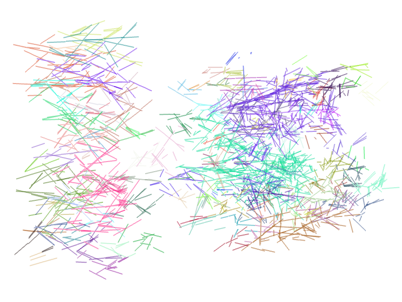
To account for both positions and directions of the track we can use the following metric: $$ \rho(\text{track}_1, \text{track}_2)^2 = || \mathbf{x}_1 - \mathbf{x}_2 ||^2 + \alpha || e_1 - e_2 ||^2. $$ Below we have the result of clustering with DBSCAN and new metric:
The clustering became much more informative: clearly, one can see now parts of the tracks, however most of the groups include more than one track, and some of the outlier basetracks are included in clusters erroneously.
Still, there is some major problem with our distance, in particular, the basetracks can be far from each other in euclidean distance and still (quite obviously) belong to a single track or shower. Metric functions used so far require that 'similar' tracks should be close in euclidean distance, and thus lost base tracks are a problem.
Alignment metric
To address named issues I introduced the following alignment distance function
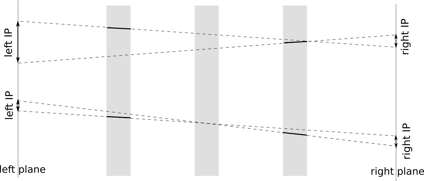
- for a couple of basetracks two planes are considered: one to the left of both tracks and one to the right
- for both basetrack intersections are found between planes and basetracks'' direction lines
- distances between intersection points $\text{IP}_1$ and $\text{IP}_2$ are computed
- distance is defined with (strictly speaking, this is not exactly distance, but DBSCAN is fine with this) $$ \rho(\text{track}_1, \text{track}_2 )^2 = \text{IP}^2_1 + \text{IP}^2_2, $$ so the basetracks are considered close when both IPs are small (which is the case when basetracks are on the same line)
- the planes selected so that both tracks are between planes and there is also some additional margin. It is needed in particular to add some distance to very close basetracks from the same layer, but with different directions
Final result
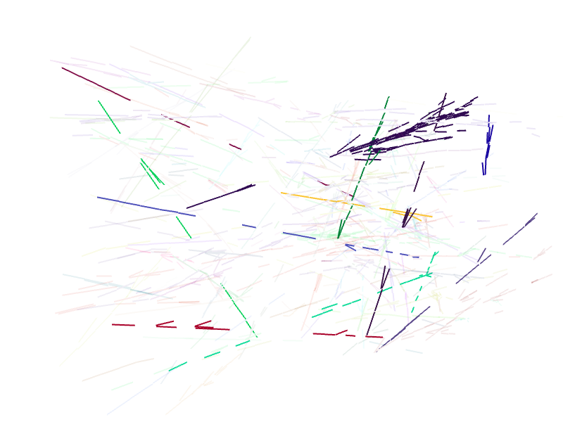
That's how alignment metric + DBSCAN perform:
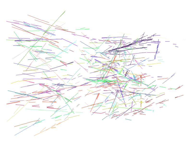
Some of the found clusters are shown in details below, you can notice that it was able to reconstruct the cluster well even when significant part of the shower is missing in the data (dark blue cluster of two parts is a single shower) or when tracks left by particles have missing basetracks in the middle
Take-home message
When data analysis approach you use relies on distance (that's almost all the clustering algorithms, but also neighbours-based methods and KDE), be sure to choose distance function wisely (using your prior knowledge about the problem), because this affects result very significantly.
References
- Demonstrations of clustering: k-means and DBSCAN by Naftali Harris
- Awesome machine learning demonstrations
- DBSCAN paper
- Blogpost with animations of clustering algorithms by Lovro Iliassich.
 Gradient boosting
  Hamiltonian MC
 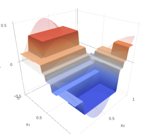 Gradient boosting
  Reconstructing pictures
 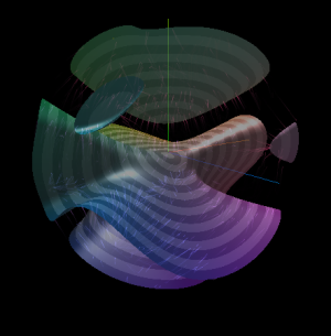 Neural Networks