Getting lost in partial derivatives
There is a nice remark from JC Baez (who writes some interesting educational thoughts about math) about counter-intuitive properties of partial derivatives:
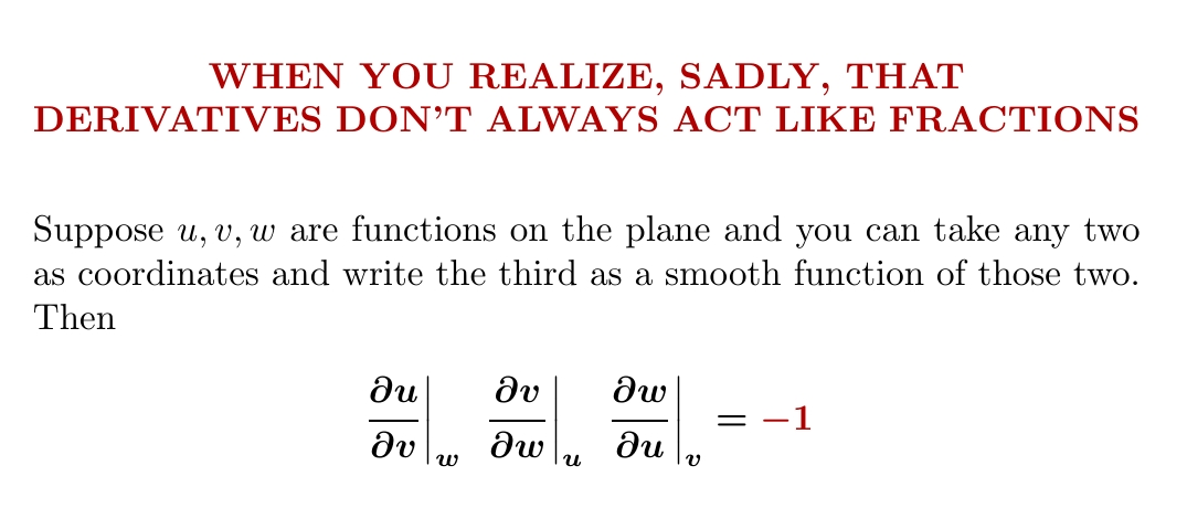 Credits: John Baez. Image is taken from the linked post
This simple example completely shatters analogy with ratios and infinitesimals that works so nicely in one-dimensional case.
There are some other problems with partial derivatives, but let’s discuss the ratio first. There are some interesting ideas how one develop an intuition for negative sign.
One of them is via differential forms:
\[\left.\frac{\partial x}{\partial y}\right|_{z} = \frac{dx \wedge dz}{dy \wedge dz}, \qquad \left.\frac{\partial v}{\partial w}\right|_{u} = \frac{dv \wedge du}{dw \wedge du}, \qquad \left.\frac{\partial w}{\partial u}\right|_{v} = \frac{dw \wedge dv}{du \wedge dv}.\]So
\[\left.\frac{\partial u}{\partial v}\right|_{w} \cdot \left.\frac{\partial v}{\partial w}\right|_{u} \cdot \left.\frac{\partial w}{\partial u}\right|_{v} = \frac{du \wedge dw}{dv \wedge dw} \cdot \frac{dv \wedge du}{dw \wedge du} \cdot \frac{dw \wedge dv}{du \wedge dv} \\ = \frac{du \wedge dw}{dw \wedge du} \cdot \frac{dv \wedge du}{du \wedge dv} \cdot \frac{dw \wedge dv}{dv \wedge dw} = (-1)(-1)(-1) = -1.\]Relations in the first line are actually super neat and are useful in a more broad context, but I’ve seen them for the first time! Above equation is based on observation that the space of 2-forms in 2d in 1-dimensional, so you can “divide” 2-forms and do this trickery with swapping multiplicants — normally this operations would be meaningless.
This proof is concise and elegant — it explains sign and generalizes to higher dimensions. Geometrically, I still lack intuition after reading it.
I find this explanation for total sign (-1) very useful: sign of
$ \left.\frac{\partial u}{\partial v}\right|_{w} $
is positive if gradients of u and v are on the same side of gradient w. In other words,
now you can plot three arrows from origin on a plane (one for each gradient) and see yourself that either one of signs is negative, or all three. When explicitly stated, you can also see this from the formula with differential forms.
Surfaces
Another interesting idea from comments to the same post is to consider 2d surface formed by (u, v, w) in 3d space.
Normal can be written as (up to coefficients, all expressions are the same vector):
\[(-1, \frac{\partial u}{\partial v}|_{w}, \frac{\partial u}{\partial w}|_{v}) \; \propto \; (\frac{\partial v}{\partial u}|_{w}, -1, \frac{\partial v}{\partial w}|_{u}) \; \propto \; (\frac{\partial w}{\partial u}|_{w}, \frac{\partial w}{\partial v}|_{v}, -1)\]and for example we can derive from proportionality of first and second vectors that \(\frac{\partial u}{\partial v}|_{w} \cdot \frac{\partial v}{\partial w}|_{u} = -1 \cdot \frac{\partial u}{\partial w}|_{v}\), and original equality immediately follows from it.
Surfaces (my approach)
Let’s consider walking along the 2d surface in 3d while keeping one of coordinates fixed. Tangent vector to our movement is proportional to one of:
\[(1, - \frac{∂v}{∂u}|_w, 0) \qquad (0, 1, -\frac{∂w}{∂v}|_u) \qquad (-\frac{∂u}{∂w}|_v , 0, 1)\]These three vectors are still in the same plane (tangent plane to the surface):
\[\det \left| \begin{matrix} 1 & - \frac{∂v}{∂u}|_w & 0 \\ 0 & 1 & -\frac{∂w}{∂v}|_u \\ -\frac{∂u}{∂w}|_v & 0 & 1 \end{matrix} \right| = 0\]and after expanding the \(\det\) one proves the original equation. Proof is “symmetric” yet still “basic”.
Now let me discuss another problem of partial derivatives: they are bulky to write (even on paper, and even more so in latex).
How a math. physicist would write partial derivatives
In mathematical physics (more of math branch rather than physics) it is somewhat common to use notation with lower indices, for example:
\[u_x = \frac{\partial u}{\partial x}|_{y} \qquad u_y = \frac{\partial u}{\partial y}|_{x}\]Noticed something? Constant clause disappears. One soon gets skilled in manipulating derivatives: \(u_\phi = u_x x_\phi + u_y y_\phi\) etc, etc
Let’s rewrite one more approach from comments. Let’s assume that surface is defined as $ f(u, v, w) $.
\[0 = df = f_u du + f_v dv + f_w dw \\ = (f_u u_v + f_v) dv + (f_u u_w + f_w) dw \\ = (f_v v_u + f_u) du + (f_v v_w + f_w) dw \\ = (f_w w_u + f_u) du + (f_w w_v + f_v) dv\]all 6 terms in brackets are zero, thus we get many relations in a form of ratio:
\[u_v = - \frac{f_v}{f_u}, ... \rightarrow u_v v_w w_u = - \frac{f_v}{f_u} \times - \frac{f_v}{f_u} \times - \frac{f_v}{f_u} = -1\]This ratio relationships are somehow more intuitive because we fixed $f$ constant.
Another notation, more common across actual physicists is operator: \(\partial_x u = \frac{\partial u}{\partial x}|_{y} \qquad \partial_y u = \frac{\partial u}{\partial y}|_{x}\)
line-saving, has no “fraction pitfall”, an easy to handle operations: \(\partial_x uv = v \partial_x u + u \partial_x v\)
Simple exercise with new notations
Consider this simple function: \(f(x, y) = y\).
\[\partial_x f = 0 \qquad \partial_y f = 1\]So far so good. How about we switch to polar coorinates? \(x = r \cos \phi \qquad y = r \sin \phi\)
\[\partial_r f = \sin \phi \qquad \partial_\phi f = r \cos \phi\]How about instead we use coordinates $(r, x)$? \(x = x \qquad y = \sqrt(r^2 - x^2) \\ \partial_x f = \frac{-x}{\sqrt{r^2 - x^2}} \qquad \partial_r f = \frac{r}{\sqrt{r^2 - x^2}}\)
And we ended up with two contradictory expressions:
\[\partial_r f = \sin \phi \leq 1 \qquad \text{and} \qquad \partial_r f = \frac{r}{\sqrt{r^2 - x^2}} \geq 1\]Answer to this riddle is very simple - just look again at the very first formula in this post. New notations do not reflect conditioning on other variables — and first expression implcitly conditions on \(\phi\) while second conditions on \(x\), hence the difference.
Approach from theoretical physicists
So how does someone who operates on coordinates all the time avoids this trap?
\[\partial_1 f = \frac{\partial f(x_1, x_2, ... , x_n )}{\partial x_1} |_{x_2, \dots, x_n} \qquad \partial_2 f = \frac{\partial f(x_1, x_2, ... , x_n )}{\partial x_2} |_{x_1, x_3, ... x_n} \qquad etc\]index implicitly assures there is “rest of variables in this pack”. And then one would casually index as such:
\[\partial_i f = \partial_i \hat{x}_i \cdot \partial_{\hat{i}} f\]Note present of hats: \(\hat{i}\) — reflects that another coordinate system is used.
This works beautifully because theorists don’t pay much attention to a particular coordinate system. It is just “plain” or “with hat” or “indexed by j” or “indexed by alpha-primed”.
Since in many partical cases you actually care about specific coordinates, your best tool is avoiding any overlaps in names between coordinate systems. Then you can safely use $\partial_x$ (and don’t fall for a “ratio” trap!).
 Gradient boosting
  Hamiltonian MC
  Gradient boosting
  Reconstructing pictures
 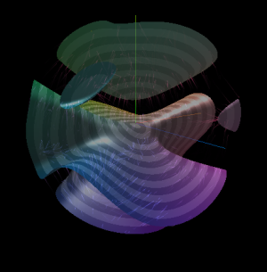 Neural Networks