Reweighting with Boosted Decision Trees
(post is based on my recent talk at LHCb PPTS meeting)
I’m introducing a new approach to reweighting of samples. To begin with, let me describe what is it about and why it is needed.
Reweighting is general procedure, but it’s major use-case for particle physics is to modify output of monte-carlo (MC) simulation to reduce disagreement with real data (RD) collected at collider.
Why do we need any simulation? When looking for rare decays, we need to train a classifier to discriminate searched particle/decay from everything else. For this purpose we use simulation of those events we expect to find in real data. Classifier is trained using this data. However, simulation is always imperfect, because it contains some approximations.
Thus we need to calibrate simulation.
For this purpose we take some well known physical process, for which there is achievable real data (real data is usually sPlot-ted to eliminate contribution of background). This process shall be close in nature to what we are looking for.
We are introducing some procedure of assigning new weights to MC such that MC and RD distributions coincide.
That’s how this looks like in simplest case:
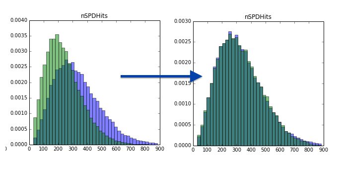
Pay attention, that the only thing we change is weights of MC distribution.
In what follows I will frequently talk about original (Monte-Carlo simulation) and target (real data) distributions.
After the reweighting rule was trained based on some normalization channel of decay, we apply it to generated simulation to get more realistic simulation results (with introduced corrections).
Typical approach to reweighting
First let’s describe how this is usually done. This method is frequently called ‘histogram reweighting’ or ‘bins reweighting’.
It is very simple, you’re splitting the features you reweighting into bins. Then in each bin you compensate the difference between MC and RD by multiplying all MC weights by a ratio:
\[\text{multiplier}_\text{bin} = \dfrac{w_\text{target, bin}}{w_\text{original, bin}}\]$w_\text{target, bin}, w_\text{original, bin}$ — total weight of events in bin for target and original distributions.
So actually, this works like dividing two histograms (another name of this method is ‘histogram division’).
What can be said about this method? This method is very fast and intuitive, however has strong limitations:
- Handles one (two if enough data) variables, almost never is able to reweight more variables.
- Reweighting one variable may bring disagreement in others, so we have to choose properly which one to reweight.
Comparison of multidimensional distributions
But before I talk about better approach to reweighting, I’d like to spend some time on comparing distributions.
Why I am interested in comparing in the context of this post? Because when reweighting samples, we want the resulting distributions to be similar and after reweighting we need to check that distributions are really close.
When there is only one variable, there are several notable 2-sample tests you can use (Kolmogorov-Smirnov, CvM, Mann-Whitney, etc.), take any of them and you’re done.
Problems start when there are two or more variables.
Checking only 1dimensional projections (which is what usually done) is not enough - that’s what you can see on the plots below. These distributions have identical 1d projections, but distributions themselves are very different:
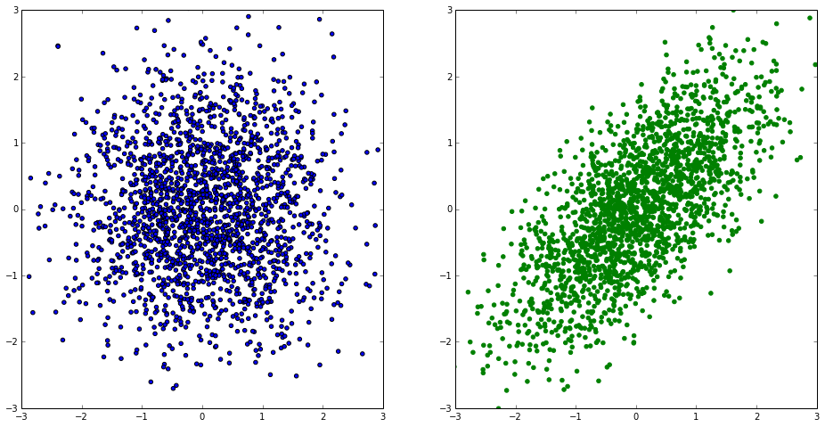
Adapting one-dimensional approaches is not of much help. Finally, there are no powerful multidimensional 2-sample tests.
The major problem here is we are trying to answer the wrong question. Two-sample tests say whether two samples of data you have were generated from same distribution.
We know that the answer is NO: simulated and real data are different.
We know this two samples are different even in the nature of appearance. The question we are interested in is whether classification model used in analysis discriminates simulation results and real data.
If not, this is good news: different numbers computed on Monte-Carlo of signal channel are reliable. You can in your computation substitute real data of signal channel (which you even can’t get with simulated).
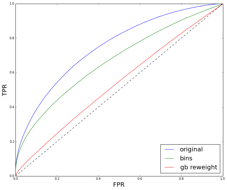
So, we need to check that classifier is not able to make a difference between RD and MC. This is simple: train a classifier to discriminate RD and MC and look at ROC curve built for test data. You shall obtain something like
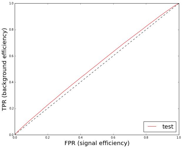
This gives you an idea of impact of disagreement between distributions to final classification quality (classification quality is checked on real background vs simulated signal). In the case this ROC curve is very high, you’re in trouble.
Caveats of reweighting
Let’s move back to reweighting with bins. Even with this simple reweighting algorithm there are some caveats, which may be not very obvious.
In this example I reweighted two variables:
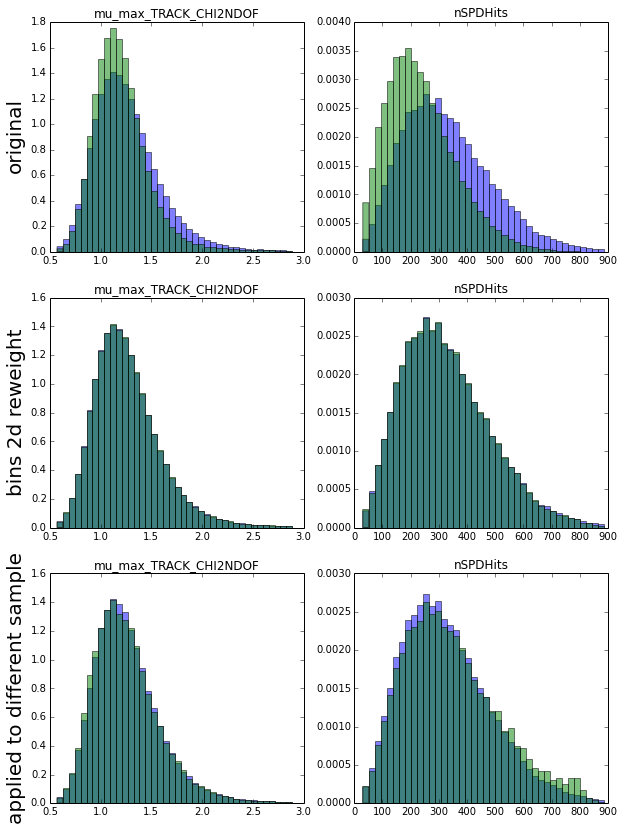
What you see above are distributions before reweighting (first row) and after (second row). After looking at result (which is second row), I see that now these distributions are in perfect match, so probably I should be very happy with this result.
But I am not, because I am interested in applying the reweighting rule to different channel. So first I test the rule on holdout — different chunk of data from the same distribution (this is third row), and I see those strange artifacts. They appeared because in some bins there were too few events and the ratio used in reweighting became vary unstable.
So the problem is in bins with few events. And we have two limit cases:
- either set very few bins (and get some harsh reweighting rule)
- or set many bins and get unstable rule.
One more note: the total amount of bins grows exponentially with dimensionality. The amount of data needed to provide stable reweighting rule grows exponentially as well.
What can we do with this?
An approach based on decision trees
The global idea is to split the space of variables into fewer regions. But this regions shall be found in some more intellectual way than just ‘split each variable into n parts’.
For this purpose we use decision trees. Recall that decision tree by checking simple conditions like $\text{feature}_i > \text{threshold}$ splits the feature space into bins, each one associated with leaf of a tree.
The remaining question is how to build the tree. We’ll greedily optimize symmetrized binned chi-squared.
\[\chi^2 = \sum_\text{bin} \dfrac{(w_\text{bin, original} - w_\text{bin, target})^2} {w_\text{bin, original} + w_\text{bin, target}}\]Note, that I want it to be as high as possible. If the weights of original and target distribution are equal, I don’t need to reweight in this bin and corresponding summand is zero. If the summand is high, reweighting in bin is needed.
Let’s visualize this:
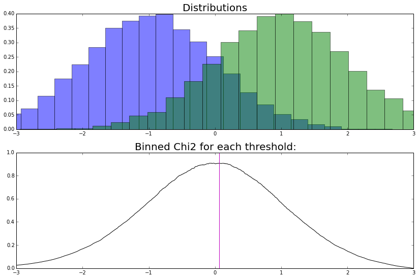
There is a simple example with two one-dimensional distributions. I am going to split this feature in two bins, so I need to find one threshold.
By checking all possible thresholds, I find out that optimal one in the sense of $\chi^2$ is right in the middle. To the left we need to decrease the weight of blue distribution, while to the right we need to increase it. Both found bins are good, and threshold seems to be close to optimal.
Since we are unable to solve global optimization problem and find optimal structure of tree, we optimize greedily, each time splitting some region to a couple of new regions (as it is usually done in decision trees).
Gradient Boosted Reweighter
Let’s move on. Gradient boosted reweighter consists of many such trees. During training we iteratively build trees, and each time reweight original distribution:
- build a shallow tree to maximize symmetrized $\chi^2$
- compute predictions in leaves:
$\text{leaf_pred} = \ln \dfrac{w_\text{leaf, target}}{w_\text{leaf, original}} $ - reweight distributions (compare with AdaBoost): \(w \leftarrow \begin{cases} w, & \text{if event from target (RD) distribution} \\ w \times e^\text{pred}, & \text{if event from original (MC) distribution} \end{cases}\)
This process is repeated many times, tree predictions are summed as usual (thus final weight, being an exponent, is obtained as product of contributions from different trees).
Note that this time we don’t have problems with few events in bins, because each tree has few large bins. Also, note that $\chi^2$ penalizes creation of bins with few events.
Let’s see how it works in practice.
In this example I reweighted 11 variables of Monte-Carlo with BDT reweighter (I also call it GB reweighter). To the left you can see original state, there is some obvious disagreement.
To the right you can see result of reweighting, and I shall admit this picture is quite boring. But after looking closer you’ll be able to see that there are still some differences.

|

|
| original distributions | after reweighting |
How about numbers?
Here is comparison of Kolmogorov-Smirnov distances for histogram reweighting and GB. Histogram reweighting was applied to the last two variables, which have high disagreement. At the same time GB reweighted all variables, and you can clearly see it by results. It even managed to get comparable results in the last two variables.
| KS original | KS bins reweight | KS GB reweight | |
|---|---|---|---|
| Feature | |||
| Bplus_IPCHI2_OWNPV | 0.080 | 0.064 | 0.003 |
| Bplus_ENDVERTEX_CHI2 | 0.010 | 0.019 | 0.002 |
| Bplus_PT | 0.060 | 0.069 | 0.004 |
| Bplus_P | 0.111 | 0.115 | 0.005 |
| Bplus_TAU | 0.005 | 0.005 | 0.003 |
| mu_min_PT | 0.062 | 0.061 | 0.004 |
| mu_max_PT | 0.048 | 0.056 | 0.003 |
| mu_max_P | 0.093 | 0.098 | 0.004 |
| mu_min_P | 0.084 | 0.085 | 0.004 |
| mu_max_TRACK_CHI2NDOF | 0.097 | 0.006 | 0.005 |
| nSPDHits | 0.249 | 0.009 | 0.005 |
Check of results
As I stressed earlier, while this one-dimensional checks are necessary, they are not sufficient.
Remember - we are not comparing one-dimensional distributions, we are checking that machine learning is not able to discriminate simulation and real data after reweighting.
And that’s what we can see. Reweighting of two variables has an effect, but this was insufficient.
Summary on gradient boosted reweighting:
So what we know about this amazing algorithm:
- BDT Reweighter many times builds trees with few but large leaves
- It is applicable to data of high dimensionality
- And when applied to same data requires less data compared to histograms method.
- On the other hand it is slow (since this is equivalent to training of GBDT), but, given that analysis lasts for months, I think we can afford ourselves to spend 5 minutes on training reweighter.
Conclusion
There are actually two major problems I covered in this post, namely comparison and reweighting of distributions. I demonstrated that both problems are addressed by machine learning.
Points you shall remember:
- check distributions using a classification model used in analysis
- check reweighting rule on a holdout
You can try reweighter, it is very simple to use:
from hep_ml.reweight import GBReweighter
gb = GBReweighter()
gb.fit(mc_data, real_data, target_weight=real_data_sweights)
gb.predict_weights(mc_other_channel)
 Gradient boosting
  Hamiltonian MC
 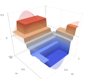 Gradient boosting
  Reconstructing pictures
  Neural Networks