Gradient Boosting explained [demonstration]
Gradient boosting (GB) is a machine learning algorithm developed in the late '90s that is still very popular. It produces state-of-the-art results for many commercial (and academic) applications.
This page explains how the gradient boosting algorithm works using several interactive visualizations.
Decision Tree Visualized
We take a 2-dimensional regression problem and investigate how a tree is able to reconstruct the function \( y = f(\mathbf{x}) = f(x_1, x_2) \). Play with the tree depth, then look at the tree-building process from above!
Explanation: how the tree is built?
First, let's revisit how a decision tree works. A decision tree is a fairly simple classifier which splits the space of features into regions by applying trivial splitting (e.g. \( x_2 < 2.4 \) ). The resulting regions have a rectangular form. In each region the predictions are constant.
Gradient boosting relies on regression trees (even when solving a classification problem) which minimize mean squared error (MSE). Selecting a prediction for a leaf region is simple: to minimize MSE we should select an average target value over samples in the leaf. The tree is built greedily starting from the root: for each leaf a split is selected to minimize MSE for this step.
The greediness of this process allows it to build trees quite fast, but it produces suboptimal results. Building an optimal tree turns out to be a very hard (NP-complete, actually) problem.
At the same time these built trees do their job (better than people typically think) and fit well for our next step.
Gradient Boosting Visualized
This demo shows the result of combining 100 decision trees.
Not bad, right? As we see, gradient boosting is able to provide smooth detailed predictions by combining many trees of very limited depth (cf. with the single decision tree above!).
Explanation: what is gradient boosting?
To begin with, gradient boosting is an ensembling technique, which means that prediction is done by an ensemble of simpler estimators. While this theoretical framework makes it possible to create an ensemble of various estimators, in practice we almost always use GBDT — gradient boosting over decision trees. This is the case I cover in the demo, but in principle any other estimator could be used instead of a decision tree.
The aim of gradient boosting is to create (or "train") an ensemble of trees, given that we know how to train a single decision tree. This technique is called boosting because we expect an ensemble to work much better than a single estimator.
How an Ensemble Is Built
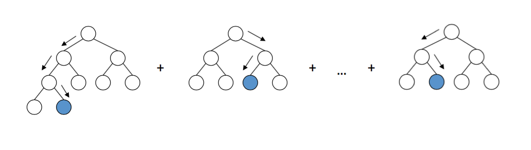
Here comes the most interesting part. Gradient boosting builds an ensemble of trees one-by-one, then the predictions of the individual trees are summed: $$ D(\mathbf{x}) = d_\text{tree 1}(\mathbf{x}) + d_\text{tree 2}(\mathbf{x}) + ... $$
The next decision tree tries to cover the discrepancy between the target function \( f(\mathbf{x}) \) and the current ensemble prediction by reconstructing the residual.
For example, if an ensemble has 3 trees the prediction of that ensemble is:
$$
D(\mathbf{x}) = d_\text{tree 1}(\mathbf{x}) + d_\text{tree 2}(\mathbf{x}) + d_\text{tree 3}(\mathbf{x})
$$
The next tree ( \( \text{tree 4} \) ) in the ensemble should complement well the existing trees and minimize
the training error of the ensemble.
In the ideal case we'd be happy to have:
$$
D(\mathbf{x}) + d_\text{tree 4}(\mathbf{x}) = f(\mathbf{x}).
$$
To get a bit closer to the destination, we train a tree to reconstruct the difference between the
target function and the current predictions of an ensemble, which is called the residual:
$$
R(\mathbf{x}) = f(\mathbf{x}) - D(\mathbf{x}).
$$
Did you notice? If decision tree completely reconstructs \( R(\mathbf{x}) \),
the whole ensemble gives predictions without errors (after adding the
Look at the plot on the right. pay attention to how the values on the vertical (y) axis decrease after many trees have been built (and the residual
becomes smaller and smaller).
After playing with this residuals demo you may notice some interesting things:
- before a tree is added to an ensemble, its predictions are multiplied by some factor
- this factor (called \( \eta \) or learning rate) is an important parameter of GB ( \( \eta = 0.3 \) in this demo)
- if we set number of trees to 10 and vary the depth: we notice that as the depth gets higher, the residual gets smaller, but it's also more noisy
- discontinuities ('spikes') appear at those points where a decision tree split
- the larger the learning rate — the larger the 'step' made by a single decision tree — and the larger the discontinuity
- in practice GBDT is used with small learning rate ( \( 0.01 < \eta < 0.1 \) ) and large number of trees to get the best results
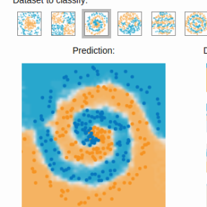
Gradient Boosting for Classification Problem
Things become more interesting when we want to build an ensemble for classification.
A naive approach that covers the difference between 'where we are' and 'where we want to get' doesn't seem to work anymore, and things become more interesting.
But that's a topic for another post.
Thanks to Micah Stubbs for proof-reading this post.
 Gradient boosting
  Hamiltonian MC
 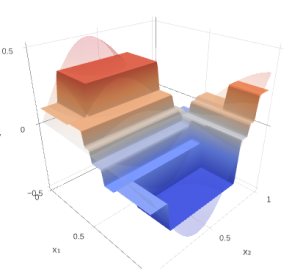 Gradient boosting
  Reconstructing pictures
 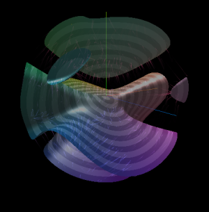 Neural Networks