Optimal control of oscillations [demonstration]
In this post I will try to briefly explain the topic and results of my PhD thesis without diving deep into mathematical explanations.
There is large family of physical processes which are described by wave equation. Most known are electro-magnetic field oscillations, acoustic waves, rod and string oscillations.
In many cases (string, rod and electro-magnetic oscillations within a wire) the process is described by one-dimensional PDE.
Controlling oscillations
In practice, modelling the process of oscillations is not enough to make us completely happy, many oscillations are harmful, and we need to stop them (in constructions/tunnels/oil pipelines/spaceships and so on).
The possible (and most practical) way to do this is to use static dumping mechanism, which will decrease energy of oscillations.
However, there is more scientific, promising way — to control oscillations by active manipulating. There are several possible ways to do this, but the one that seem to be implementable in practice with least efforts is boundary control.
As an example of problem setting in this approach: provided that I'm observing oscillations of a string, I want to dump those as soon as possible. I can do this by applying forces at the ends of the string (or only from one side), so I have to define the functions $\mu(t), \nu(t)$, which describe the dependency of applied force on the time. $\mu(t), \nu(t)$ correspond to left and right ends of a string.
The information I have is initial state of the string (described by string profile and profile of its velocity), and a desired final state (again, described by a pair of functions). This general case is reduced in a straightforward way to the excitation problem, when initially the string rests (profile shift = 0, velocity = 0), but the final state is still arbitrary (profile shift = $\varphi(x)$, velocity = $\psi(x)$).
Standard approaches to control oscillations
An optimal control theory, which was initially developed for finite-dimensional systems, cannot be applied directly to this problem, but there are several ways to overcome the limitation by using different discretizations of this problem. Many papers were devoted to this approach, and to fighting appearing problems (see papers of Zuazua E. and his co-authors). Probably, first systematic (and quite general) way to handle excitation/dumping problems was Hilbert Uniqueness Method (HUM) proposed by J.-L. Lions.
While being quite general, this approach leads to linear system on function argument, which still should be solved approximately.
Analytical approach to control oscillations
Another approach is to use analytical computations: solve explicitly mixed problem, express final state as an a function of boundary conditions and then rewrite final conditions as a system of functional equations + optimization problem. Solve it (again, analytically).
This approach was applied by Vladimir Il'in (rus: академик Владимир Ильин). It is not obvious that such computations are possible in explicit way, but in the case of wave equation (and very few others) this is doable.
My contribution and result
I was able to generalize the approach to the case of system of rods/strings, connected sequentially. This required some beautiful math, the method is based on operator matrices.
Resulting formulas are not very easy to follow, but they are really fast (most resources in this demo are spent on drawing, not computing) and quite general (compared to previous analytical results). This approach is able to work with arbitrary pair of boundary conditions of first/second kind (and also supports fixed or free boundaries, but I didn't add this into demonstration interface).
Now we pass to interactive demonstration of this approach to control vibrations.
Optimal control of oscillations in system of rods / strings explanations
Function |
Target shiftTarget velocity |
System parametersControl time set is equal to critical time, so the control is performed up to global shift. If you want to have complete control, please increase control time. Control time set is less that critical, control is impossible. |
Explanations
This page is a demonstration of results on analytical controllability of rod oscillations (or string oscillations, which is the same), presented in the following papers:
- Alex Rogozhnikov, Study of a mixed problem describing the oscillations of a rod consisting of several segments with arbitrary lengths [rus, en]
- Alex Rogozhnikov, Optimal control of longitudinal vibrations of composite rods with the same wave propagation time in each part [rus, en]
- Alex Rogozhnikov, On different boundary conditions [only in russian]
Formal setting
There is a system of rods, which initially rests. There are $n$ parts in the system, each having constant density $\rho_i$ and Young's modulus $k_i$ (each part is made of some material).
The goal is to produce such boundary control functions $\mu(t), \nu(t)$, which will drive the system to the fixed final state, defined by shift $\phi(x)$ and velocity $\psi(x)$ as the moment $T$ (time of control).
Suppose that time spent by wave to pass each part equal (for simplicity we also use $T$ proportional to this time). Since there are infinitely many solutions of this control problem (for the exception of some situations), we look for controls that minimize so-called boundary control energy.
How to use the demo
Enter parameters of a problem:
- Set the number of parts in rod, for each part enter its density $\rho_i$ and Young's modulus $k_i$ for each of the parts.
- Set the functions $\varphi(x), \psi(x)$. Pay attention, that values are taken from $[0 \leq x \leq 1]$ and linearly stretched.
- Select boundary conditions (first/second kind).
Or press 'generate problem' button — then it will choose all the parameters randomly.
Press 'Go' and enjoy the process. On the left plot green line is shift $u(x, t)$, grey is velocity $u_t(x, t)$. Computed control function $\mu(t)$ and $\nu(t)$ are displayed on the plots in the middle column. There are three lines on each plot corresponding to three values $y=0,+1,-1$ to demonstrate scale.
Developed in 2013.
 Gradient boosting
 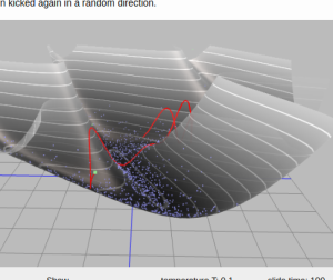 Hamiltonian MC
  Gradient boosting
  Reconstructing pictures
 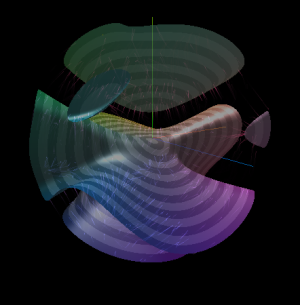 Neural Networks