Data manipulation with numpy: tips and tricks, part 1¶

Some inobvious examples of what you can do with numpy are collected here.

Examples are mostly coming from area of machine learning, but will be useful if you're doing number crunching in python.

1. numpy.argsort¶

Sorting values of one array according to the other¶

Say, we want to order the people according to their age and their heights.

once you computed permutation, you can apply it many times - this is fast.

Frequently to solve this problem people use sorted(zip(ages, heights)), which is much slower (10-20 times slower on large arrays).

Computing inverse of permutation¶

permutations in numpy are simply arrays:

Inverse permutation is computed using numpy.argsort (again!)

This is true because of two facts:

1. indexing operation is associative (dramatically simple and interesting fact):

   a[b][c] = a[b[c]]

   provided that a, b, c are 1-dimensional arrays

2. `permutation[inverse_permutation] is identical permutation:

Even faster inverse permutation¶

As was said, numpy.argsort returns inverse permutation, but it takes $O(n \log(n))$ time, while computing inverse permutation should take $O(n)$.

This optimal way can be written in numpy.

Computing order of elements in array¶

frequently it is important to compute order of each value in array.

In other words, for each element in array we want to find the number of elements smaller than given.

NB: there is scipy function which does the same, but it's more general and faster, so prefer using it:

IronTransform (flattener of distribution)¶

Sometimes you need to write monotonic tranformation, which turns one distribution into uniform.

This method is useful to compare distributions or to work with distributions with heavy tails or strange shape.

Let's apply Iron transformation to data

Now we can see that IronTransform actually was able to turn signal distribution to uniform:

How IronTransform works¶

To turn any distribution into uniform, you should use mapping: $x \to F(x)$, here $F(x)$ is cumulative distribution function.

In other words, for each point $x$ we should compute the part of distribution to the left. This was done by summing all weights to this point using numpy.cumsum (we also had to normalize weights).

To use the learned mapping, linear interpolation (numpy.interp) was applied. We can visualize this mapping:

IronTransform and histogram equalization¶

The same method is applied in computer vision to 'improve' low-contrast images and called histogram equalization.

Also worth mentioning: to fight very small / large numbers, use numpy.clip. Simple and very handy:

2. Broadcasting, numpy.newaxis¶

Broadcasting is very useful trick, which simplifies many operations.

Weighted covariation matrix¶

numpy has cov function, but it doesn't support weights of samples. Let's write our own covariation matrix.

Let $X_{ij}$ be the original data. $i$ is indexing samples, $j$ is indexing features. $COV_{jk} = \sum_i X_{ij} w_i X_{ik}$

alternative way to do this is via numpy.einsum:

Pearson correlation¶

One more example of broadcasting: computation of Pearson coefficient.

Pairwise distances between vectors¶

we're given a set of vectors (say, 1000 vectors). The problem is to compute their pairwise distances.

also, since algebra is you friend, you can do it times faster: $$||x_i - x_j||^2 = ||x_i||^2 + ||x_j||^2 - 2 (x_i, x_j) $$ so dot products is the only thing you need.

... but keep in mind there is sklearn.metrics.pairwise which does it for you and has different options

3. numpy.unique, numpy.searchsorted¶

Converting categories to small integers¶

Despite categories are easier to read, operating with them is much faster after you represent them as small numbers
(for instance, in range [0, n_categories - 1])

First generate some categories:

Now we use numpy.unique to convert them to numbers (pay attention to return_inverse=True)

Also we can reconstruct old categories if needed:

Mapping new categories¶

When we need to map new categories using the same lookup table, we can use numpy.searchsorted

Checking values present in the lookup¶

Usually, we use set to have many checks that each element exists in array. But numpy.unique is better option - it works dozens times faster.

Handling missing categories¶

When some new category appears in test data, this is always a trouble. Possible solutions:

• map randomly to one of present categories (this, i.e. is done by hashing trick)
• make a special category 'unknown' where all new values will be mapped. Then special value may be chosen for it. This approach is more general, but requires more efforts.

Below you can find the transformer for second approach:

4. numpy.percentile, numpy.bincount¶

Splitting data into bins¶

Splitting data into bins is frequently necessary. Simplest way done e.g. by numpy.histogram is splitting region with even bins of same size.

This usually works poorly with distributions with long tails (or strange shape) and requires additional transformation to avoid empty or too large bins.

However, for most cases creating the bins with equal number of events gives more convenient and stable results. Selecting the edges of bins can be done with numpy.percentile.

the number of events within each bin is equal now.

Defining the index of bin¶

Use numpy.searchsorted to compute the index of bin for each value in x. (numpy.digitize is the other option, it does the same).

numpy.searchsorted assumes that first array is sorted and uses binary search, so it is effective even for large amount of bins.

Counter¶

Need to know number of occurences for each category? Use numpy.bincount to compute the statistics:

This will compute how many times each category present in the data:

the same done with collections.Counter (which is much slower)

Replace category with number of occurences¶

There are several tricks important to process the categorical features. Most known one is one-hot encoding, but let's speak about others.

One of tricks is to replace in each event category (which cannot be processed by most algorithms) with a number of times it presents in data.

This can be written in numpy one-liner:

Averaging predictions over category¶

Another important trick: replace category with average prediction for events from this category.

This is more tricky, since we need to add weights to numpy.bincount:

Variation of predictions over category¶

The same trick can be applied to measure deviation after invloving some math: $$ \mathbb{V}x = \mathbb{E}x^2 - (\mathbb{E}x)^2 $$

You can also assign weights to events and compute weighted mean / weighted variation using the same functions.

5. Numpy.ufunc.at¶

To proceed futher, we need to know that there is class of binary (and unary) functions: numpy.ufuncs

Examples: numpy.add, numpy.subtract, numpy.multiply, numpy.maximum, numpy.minimum

In the following example we cook a new column with maximal predictions over category using ufunc.at

Important note: numpy.add.at and numpy.bincount are very similar, but latter is dozens of times faster. Always prefer it to numpy.add.at

Multidimensional statistics: numpy.add.at and smart indexing¶

When need to compute number of times each combination met, there are two ways:

1. convert couple of variables to new variable, e.g. by feature1 * (numpy.max(feature2) + 1) + feature2
2. create multidimensional table

I prefer first, code below is demonstration of second approach and it's benefits.

Now some useful things we can do with colected statistic. First thing is create feature, for which we use fancy indexing:

We can also infer different statistics like:

• you are not limited to numpy.add, remember there are other ufuncs.
• Few space to keep whole matrix? Use scipy.sparse if there are too many zero elements. Alternatively, you can use matrix decompositions to keep approximation of matrix and compute result on-the-fly.

Computing ROC curve¶

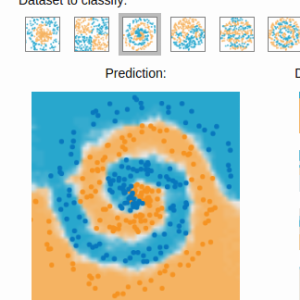
As an important exercise, let's implement the computation of ROC curve. (interactive demo of ROC curve may be found here )

We will write the same as sklearn.metrics.roc_curve (actually, simplified version of it).

ROC curve takes three arrays: labels (binary, 0 or 1), predictions (real-valued) and weights.

Let's check how result looks like:

Weighted Kolmogorov-Smirnov distance¶

ROC curve is an important object by itself and freqently used in ML to compare distribution, but the magic is that it contains all order-based information about original distributions.

Next we compute KS distance based on ROC curve:

$$ KS = \max_x \left| F_1(x) - F_2(x) \right| $$

(Order-based information == information, which is preserved under monotonic transformations)

Compare results with standard function:

Important moment that written function supports weights, while scipy version doesn't.

TODO: optimal F1, optimal accuracy based on ROC curve.

Conclusion¶

Many things can be written in numpy in efficient way, moreover resulting code will be short and (surpise!) more readable.

But this skill requires much practice.

See also¶

• Second part of post: numpy tips and tricks 2
• I used example from histogram equalization with numpy
• Numpy log-likelihood benchmark